Problems 2.7 Assessing Model Performance
- Rework problem 2.4 exercise 2, but restrict the data to a single year. For example, just use data after August 1st, 2014.
gflu = read.csv("https://raw.githubusercontent.com/EcoForecast/EF_Activities/master/data/gflu_data.txt",skip=11)
time = as.Date(gflu$Date)
y = gflu$Massachusetts
yobs = y[time > "2014-08-01"]
tobs = time[time > "2014-08-01"]
plot(tobs,yobs)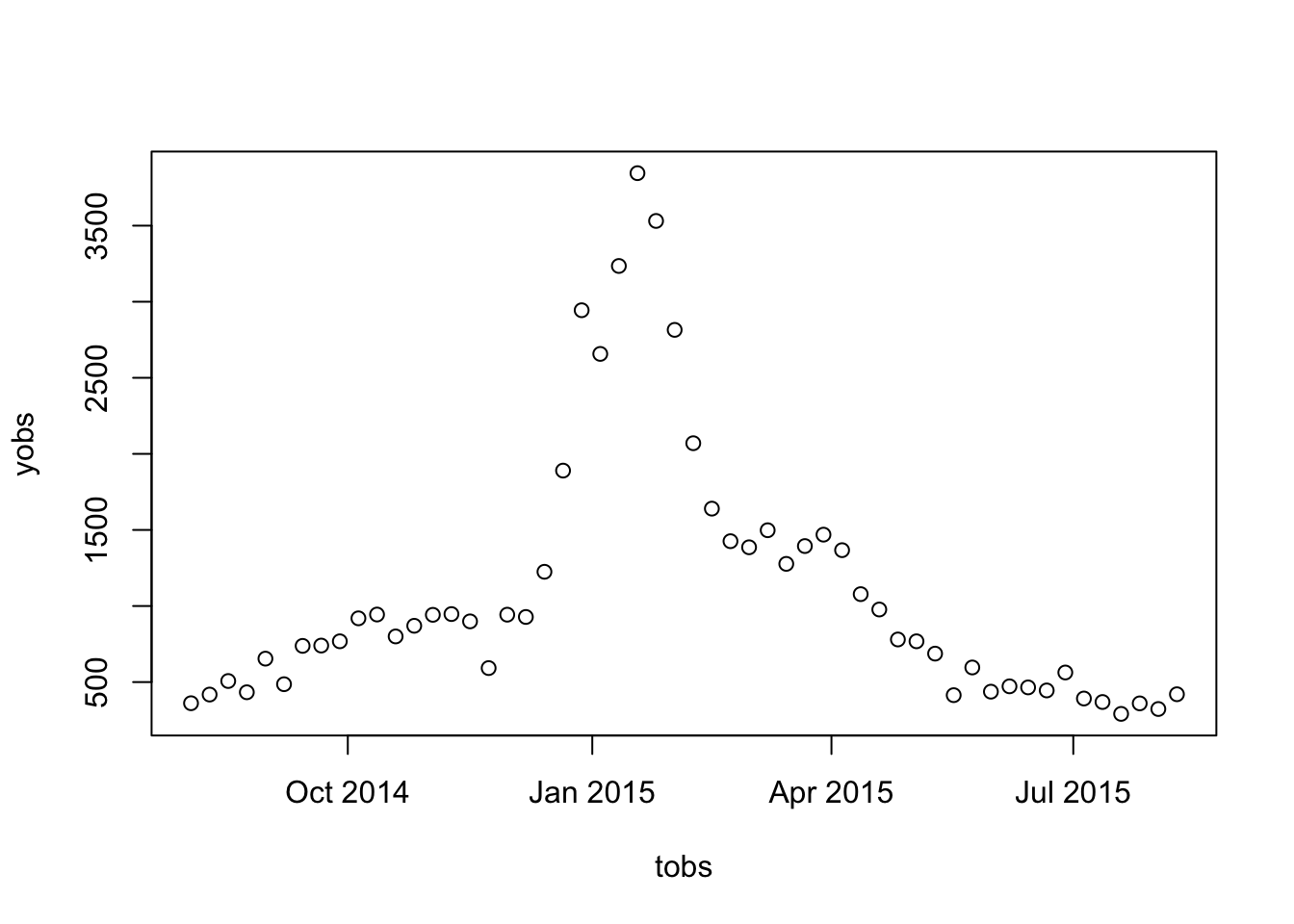 Create various visualizations to assess model performance as per the suggestions in Dietz, chapter 16. As a minimum, (1) plot the mean model output along with the observed cases vs time, (2) plot observed vs predicted (mean) and compute the correlation \(R^2\), and (3) plot the residuals (observed less predicted) vs both time and predicted. Comment on the results.
- (optional) Create visualizations and compute descriptive statistics to assess the model of problem 2.5 or any model used in any other problem sets in the school (I.e., pick your favourite model and assess it).