8 Entering and loading data
8.1 Entering data
Good data organization is the foundation of any research project, and this begins with entering and archiving data. More detail on the practice of good data entry and documentation can be found in Chapter 12. This chapter focuses on the “how to” of data entry in R.
There are several reasonable options for data entry, for example:
- Spreadsheet
- Text file
- Database
- Form (web or GUI databases).
In R, you can also input data directly, which can be the right choice if you are working with a small dataset. Here, you will learn how to enter the data from your experiments and save them using R.
Let’s start by
making Table 1 for your report, which we will call
solution-concentration-effect-on-potato.csv:
table1 <- data.frame(weight = c("initial", "final",
                                "difference", "percent-change"),
                     "NaCl-0-percent" = c(NA, NA, NA, NA),
                     "NaCl-0.9-percent" = c(NA, NA, NA, NA),
                     "NaCl-2-percent" = c(NA, NA, NA, NA),
                     "NaCl-5-percent" = c(NA, NA, NA, NA))
write.csv(x = table1, file = "solution-concentration-effect-on-potato.csv",
          row.names = FALSE)
In the above code, make sure to replace the NA’s with the values from your experiment.
Keep in mind that the values entered into the tables should be
decimals greater than or equal to zero, and likely less than
100 since you measured mass in grams and the potato
cubes for the experiments were 8 cm3 in size.
Notice that we used the file extension “.csv”. CSV stands for comma-separated values, which is a format for tabular data stored in a text file where a comma separates the columns of the data. That is why a comma separates each of the values in the rows for the different solutions.
Now, we will make Table 2, which includes the class averages and we will call
solution-concentration-effect-on-potato-averages.csv:
table2 <- data.frame(weight = c("percent-change", "minimum-value",
                                "maximum-value", "difference"),
                     "NaCl-0-percent" = c(NA, NA, NA, NA),
                     "NaCl-0.9-percent" = c(NA, NA, NA, NA),
                     "NaCl-2-percent" = c(NA, NA, NA, NA),
                     "NaCl-5-percent" = c(NA, NA, NA, NA))
write.csv(x = table1, file = "solution-concentration-effect-on-potato-averages.csv",
          row.names = FALSE)
You might have just done this in Excel. We did not teach this method because Excel is not recommended for data entry. There are compatability issues between Excel and R that create problems. Spreadsheet software like Excel can be handy for data entry, but you should think carefully about how to organize your rows and columns first (see Chapter 12 for details). If you do have data in Excel, you should convert it to a .csv (comma delimited format) first, before you import to R.
Here are two articles that do a nice job discussing the differences and pros/cons of Excel vs. R
Excel v R: read the first section only
8.2 Loading or importing data
We will look at three ways of importing data into R: 1) via a command, 2) using the import feature, or 3) directly from the internet. The first two options are equivalent. The third option is easier but requires an internet connection. When they are successful you will see your data as a new object in the Environment tab (in the Environment/History pane).
8.2.1 The programmatic way (i.e., command line)
We can load our our data files in CSV format into R using the function read.csv in the following way:
data1 <- read.csv(file = "solution-concentration-effect-on-potato.csv")
data2 <- read.csv(file = "solution-concentration-effect-on-potato-averages.csv")
Here, the argument file = of read.csv is the name of the file we want to read.
Notice that the filename needs to be a character string, so we put it in quotes.
This method is the best way to import your data, however depending on your familiarity with your computer’s file structure you may spend quite some time determining how to the call the path to where you have saved your .csv file.
8.2.2 The RStudio way (the “import” feature)
In RStudio, click on the Environment tab.
Then, click on Import Dataset and select From Text (base).
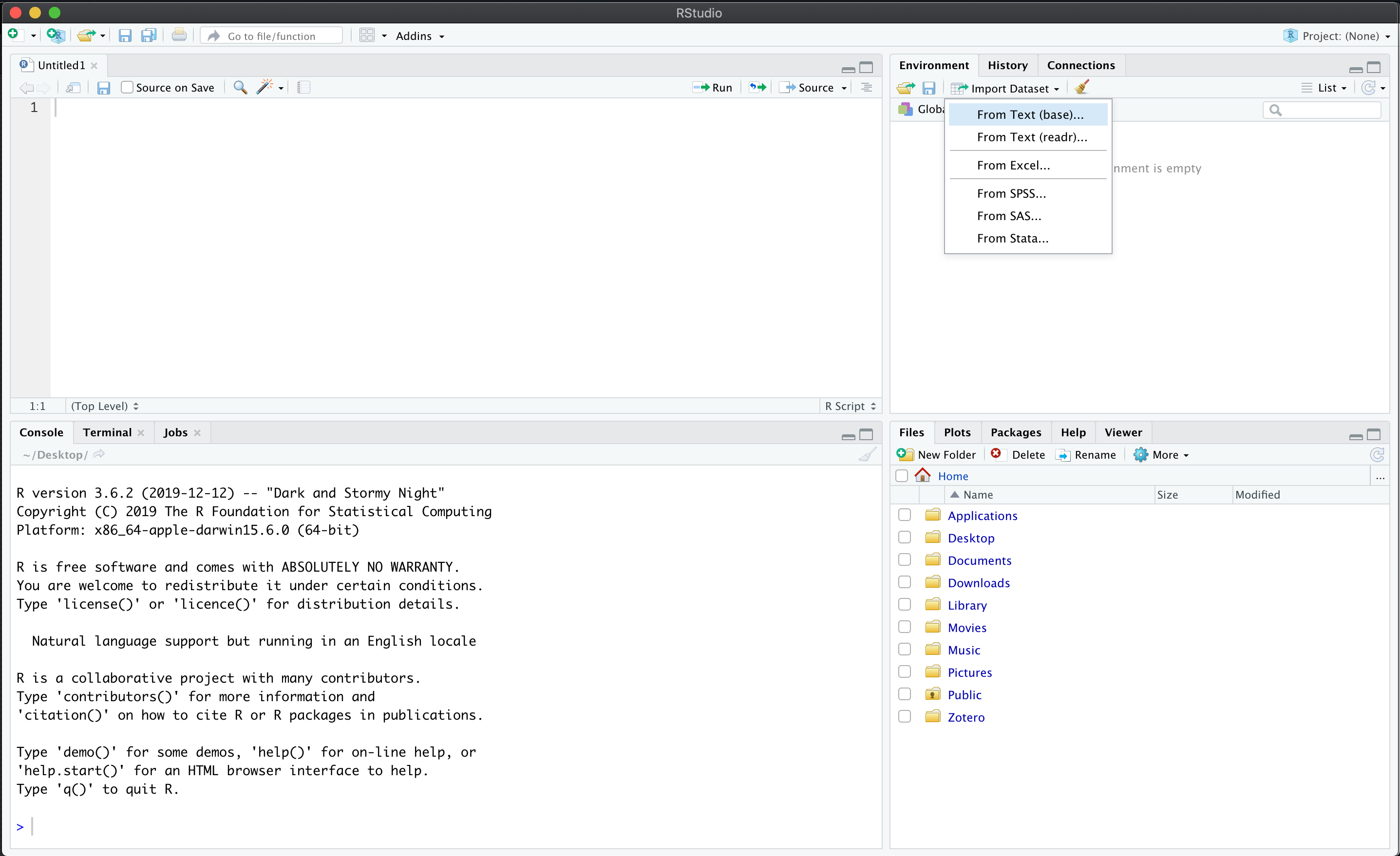
Figure 8.1: Using the Import Dataset feature.
This feature will open a file browser where you can locate the .csv file,
in our case, for Table 1, it is called solution-concentration-effect-on-potato.csv.
Once you have selected the file click Open.
A dialog for importing the file will open up:
on the left you can set the options on the import;
on the top right you can see Input File, which is how the file looks like;
on the bottom right you can see Data Frame,
which is a preview of how the file or data will look like in R.
In the Name field, write data1 to rename the dataset.
Set Heading to Yes, this will
tell R to read and include the first row of the file as the names of the columns -
This is an important step!
You will see that the column names appear in bold in the Data Frame box.
When you are ready click Import.
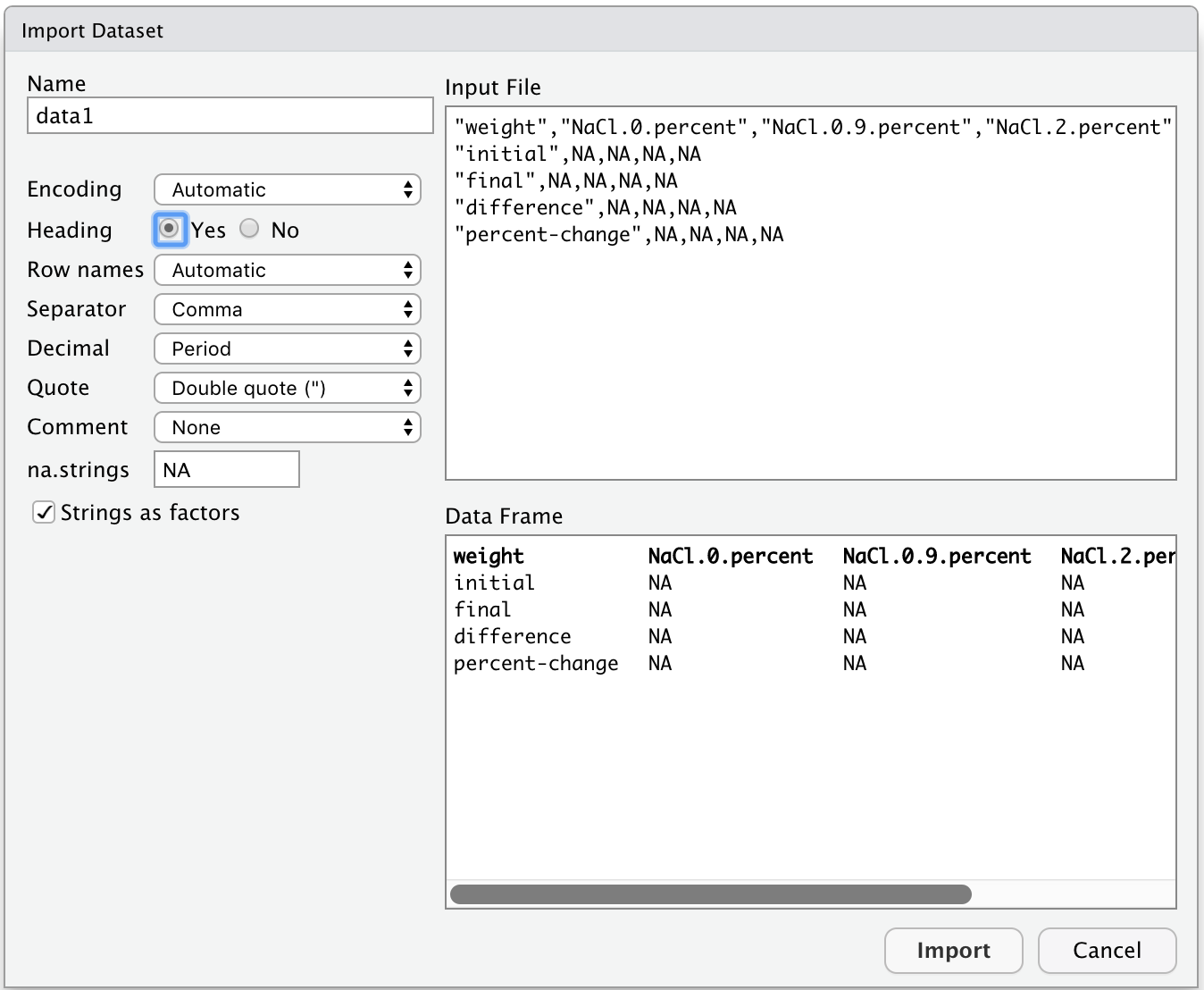
Figure 8.2: Dataset import options.
RStudio will now run the R code that imports your dataset. It will be similar to the command used in Section 8.2.1.
8.2.3 Loading data hosted on a url
For Memorial University biology courses we try to host data on the internet so that it is easy to import data when there is an internet connection.
For example, the Falik et al. data that is used in BIOL 1001 can be loaded using this command:
Falik.Data = read.csv("https://raw.githubusercontent.com/ahurford/quant-guide-data/main/BIOL1001-data/FalikDataset.csv")You can copy and paste this code into your Console or Script and if you have an internet connection the data will load.
Data that we know is used in Biology courses at Memorial are hosted here. If you are a Memorial University instructor and would like to add your data, please email ahurford-at-mun.ca.
To find the correct url, you should navigate through the folders to the data source that you are interested in, then click the Raw button.
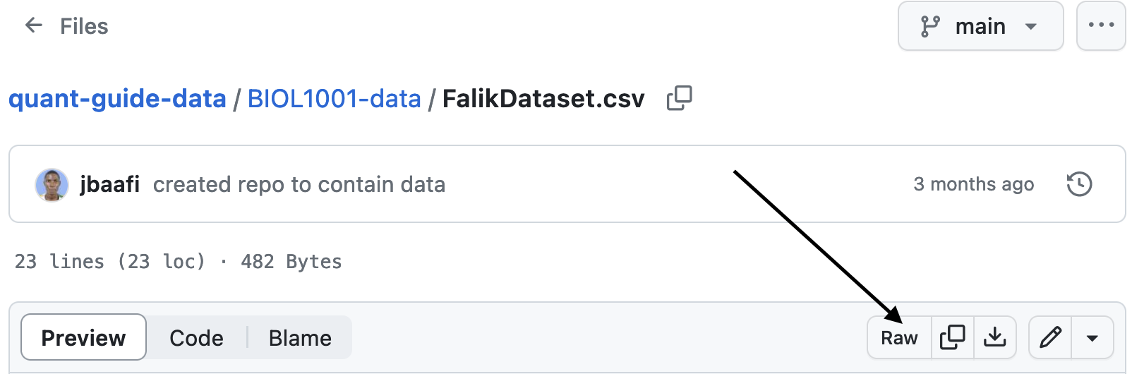
Figure 8.3: The raw button for data hosted on Github.
This will navigate to the url that you can copy and paste into your R script. For the example above, this is: https://raw.githubusercontent.com/ahurford/quant-guide-data/main/BIOL1001-data/FalikDataset.csv
This approach to loading data can be vastly easier for beginners, however, it requires that the data is appropriately hosted on the internet (which may not always be the case) and so eventually learning the one of the other two methods is recommended.
8.3 Inspecting the data
To take a look at our dataset, we can print it by typing the name in the Console and hitting Enter (or Return).
##           weight NaCl.0.percent NaCl.0.9.percent NaCl.2.percent NaCl.5.percent
## 1        initial             NA               NA             NA             NA
## 2          final             NA               NA             NA             NA
## 3     difference             NA               NA             NA             NA
## 4 percent-change NA NA NA NA## weight NaCl.0.percent NaCl.0.9.percent NaCl.2.percent NaCl.5.percent
## 1 initial NA NA NA NA
## 2 final NA NA NA NA
## 3 difference NA NA NA NA
## 4 percent-change NA NA NA NAYou can also open the dataset by clicking on the object data1 in the Environment tab.
This will open a new tab with the dataset, instead of printing it into the Console,
which is a good choice if your dataset is larger.
Another option is to open the dataset using Microsoft Excel from your computer file browser.