3 Finding your way around RStudio
RStudio has 4 windows (also known as “panes”) that are inter-linked. The default layout is shown in Figure 3.1. The first time you open RStudio you may not see the top left pane (the Source pane, labeled 2 in the figure below). To make it visible, use your mouse to select File -> New File -> R Script. You can move the layout of the panes and change their size and shape by clicking and dragging with your mouse along the windowpane borders. The details of what happens in each pane are detailed below.
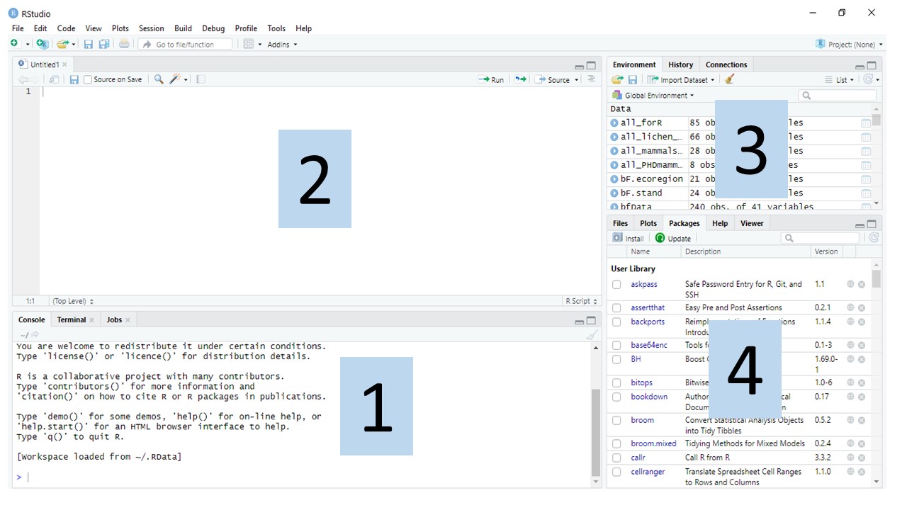
Figure 3.1: Panes in RStudio. 1. Console pane, where code is executed by R. 2. Source pane, to work with R scripts (code won’t be evaluated until you send it to the console). 3. Environment/History pane, to view objects in the working space and command history, respectively. 4. Files/Plots/Packages/Help pane, to see the file directories, plots, installed packages and access R help, respectively.
3.1 Console pane
The Console pane (labeled 1 in Figure 3.1) is where code is evaluated (also referred to as executed). The Console pane has a prompt (the > symbol), which tell you that R is ready to receive input. You can type code here to evaluate it and get an output.
TRY IT! Type 5 + 5 in the console at the prompt and press enter or return. You’ll see that R gives the correct output (Don’t worry about the [1] for now, we’ll discuss what this means later.
## [1] 10Use the console to test and query code, or do a quick analysis that you do not want to save. Press the up arrow to scroll through past commands, from most to least recent.
To do more interesting things, we need to assign values to objects. For this, we create an object by specifying a name followed by the assignment operator <- and the value we want to give it. For example:
When you run this code by pressing enter/return you will not see an output as you did before. But, you can ask R for the value by typing the object name and pressing enter/return:
## [1] 5Now that we have saved the value of x, we can do arithmetic operations with it. For example, instead of adding two numbers, we can assign those values to objects and then add them.
TRY IT! Add 3 and 8 by assigning the values to objects. First assign 3 to x and 8 to y. Then add x+y.
You can overwrite the value of objects The current value of your object is the last value you gave it. In the console type:
Press enter/return. Now type:
Press enter/return. What is the value of
## [1] 2Type:
## [1] 1to query the current value of x.
EXCERCISE
Can you write the code, and execute the commands in the correct order so that x + 1 = 6?
3.2 Source pane
The Source pane (labeled 2 in Figure 3.1) is where you create, save, and edit R scripts. R scripts are blocks of code that perform a task that you want to save (e.g.., are the answer to the EXERCISE above, or import and clean data to make a figure) and when saved have a .R extension. When you’ve written and saved a script, you can re-use it for future projects. Try it now: open and save a new .R file to save your work in. In the top menu select File > New File > R Script, then File > Save As. Paste the following R code into your script and save it:
x <- 4
x <- 6
Now, you have saved this code, but has it been evaluated? To answer this question type x in your Console and press ENTER:
## [1] 1It is important to note that saving commands in a script in your Source window does not evaluate the commands in your Console. To execute the commands, with your script displayed in the Source pane, you need to click the Source button (righthand side of the source pane, equivalently select Code > Source from the top menu bar; note, if you have a small Source pane the Source button may not appear and you may need to make it bigger or use the menu bar).
Source your script and then evaluate x in your Console. If you have done this task correctly the value of x should be 6 and it will appear as [1] 6 in your Console.
What happened to x <- 4? When Source is called the commands are executed in the Console from top to bottom as they appear in the script. Therefore, x <- 4 was only the current value of x for a very short time before it was overwritten with the command x <- 6.
EXERCISE
Edit your script so that now it reads:
x <- 4
y <- x + 1
x <- 6
z <- x + 1
Source the script and then query the values of y and z in your Console. What are the values returned for y and z? Explain how these values were returned.
> y
> z
If you would like to run one line or several lines of your script only (not all the lines), then place your cursor on the line you want to execute and click the Run button (equivalently Code > Run Selected Line(s), or press Ctrl+enter or Cmmd+return for a shortcut).
3.3 Environment/History pane
This pane has several tabs, we’ll discuss each in turn.
Environment tab
This shows you the names of all data objects (e.g., vectors, matrices, data frames) that you’ve defined in the current R session, along with information about the size of data objects.
There are also clickable actions, like Import dataset, which we’ll refer to in Chapter 8.
History tab
This shows you a history of all the code you’ve previously run in the console. From here you can re-run these commands by selecting them and clicking To Console or include them in your script by clicking To Source.
TRY IT! Select one of the commands and click To Console. You’ll see the command is executed and the output is given. Now, try to include another command in the script that you have been working with during this session.
3.4 Files/Plots/Packages/Help/Viewer pane
This pane also has a few tabs. We’ll go through each one in detail.
Files tab
This tab gives you access to the file directory on your own computer. It’s a useful spot to set your working directory. For this, you have to navigate to the folder whence you want to read and save files, then click More and select Set As Working Directory (see Chapter 8 for more details).
TRY IT! Navigate through the file tree and find the folder that you want to work with, alternatively, create a new one by clicking New Folder. Now, open the folder and make it your working directory. You’ll see that in the console R runs the command for changing the working directory.
Plots tab
This tab lets you see all the plots (graphs) that you create. You can also use the buttons at the top to zoom or export the graph as a PDF or jpeg file. If you make multiple plots, you can navigate through them by clicking on the left and right arrows. We will come back to this tab in Chapter 10.
Packages tab
This tab shows a list of all the R packages installed on your computer (see Chapter 4 for more on packages). It also indicates which packages are currently loaded via a check mark. You can browse through the installed packages by typing the name in the blank search field. Packages are add-on functions and data sets that you can add to your R installation.
More information about on Packages can be found in section 4.10 R Package.
TRY IT! One package that we will use later on is called ggplot2, install it either using the install.packages command or the Install feature.
Help tab
Here you can get help with R functions. You can type the name of the function in the search field (blank bar with the magnifying glass beside it) to see the related help page. Equivalently, you can use code to perform the search by typing ? followed by the function name. See Chapter 5 “Getting R help” for more details on reading the help files.
TRY IT! Find the help page for the plot function, either by typing the function name in the search field or directly into the console. You can type it directly into the console via ?plot command. We will use this function in Chapter 10.