17 R markdown
17.1 Introduction
R Markdown provides a fully reproducible framework for presenting and sharing data science. You can use a single R Markdown file to both:
- save and execute code
- generate high quality written documents
R Markdown documents can be rendered to many output formats including HTML documents, PDFs, Word files, slideshows, etc.
17.2 Setup
To get started, open a new text file and save it with the extension .Rmd. Alternatively, if you are using RStudio, you can create a new Rmd file from the menu File -> New File -> R Markdown.
An R Markdown file contains three types of content:
An optional header that contains the document metadata and is surrounded by
---on either side.Chunks of R code surrounded by
```and specifying{r}at the top.Text that is easily formatted
In general, your R Markdown file will look like this when using RStudio.
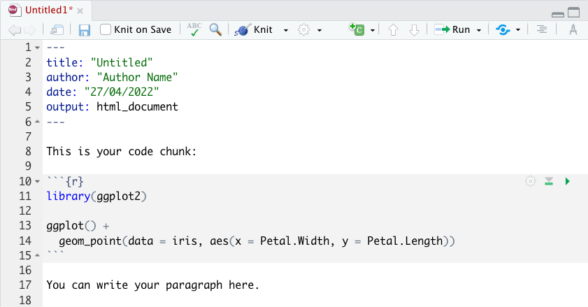
Figure 17.1: R Markdown general setup
The header is written using YAML programming language. R Markdown files are often set as html documents and can be changed to a PDF or word document at any time. Alternatively, they can immediately be specified as word_document, etc.
You can run each code chunk by clicking the Run icon or small green triangle at the start of each chunk. RStudio executes the code and displays the results inline with the code. If you want to prevent the source code from being displayed, you can set {r, echo = FALSE} at the start of the code chunk.
Note that text is written as you would in any word processing program, unlike .R files where you need to comment text using the pound symbol (#).
Tip: Try to leave at least one empty line between adjacent elements, e.g., between a header and a paragraph or between text and code, to ensure everything renders properly.
17.3 Rendering to a document
To render your R markdown file into an HTML, PDF, or Word document, click the “Knit” icon that appears above in the bar above the source pane. This will automatically render your document to the output format specified in your header, however, the drop down menu will allow you to select an alternative type of output.
Once the file is rendered, RStudio will show you a preview of the new output and save the output file in your working directory.
Here is an example of how the markdown script above would look un a HTML output format.
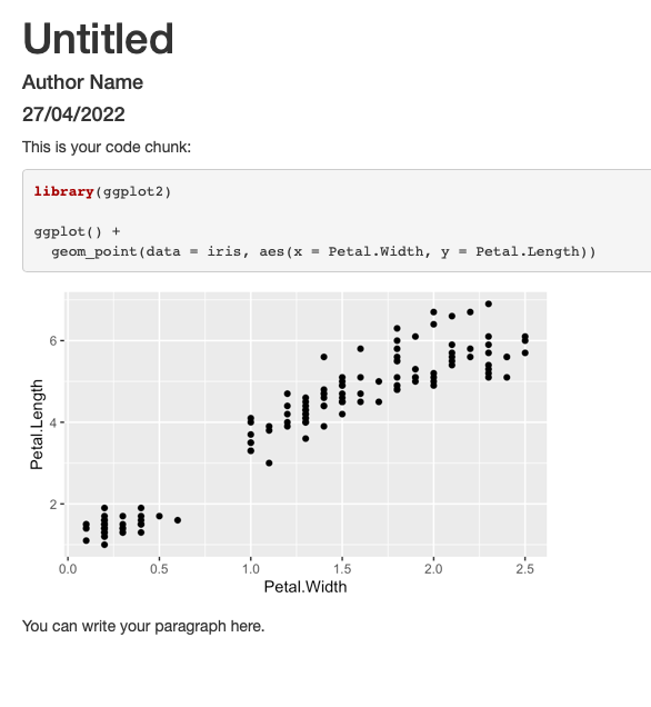
Figure 17.2: R Markdown output preview
17.4 Formatting
17.4.1 Syntax
It is very easy to modify your inline text. Italic text is produced by surrounding words with underscores or asterisks, e.g., _italic_ or *italic*. Bold text is produced with a pair of double underscores or asterisks, e.g., **bold** or __bold__.
Superscripts are produced using a pair of carets (^), while subscripts require a pair of tildes (~), e.g. superscript^2^ = superscript2 vs subscript~2~ = subscript2.
17.4.2 Headers
Section headers can be written after one or more pound signs (#), where increasing the number of pound signs increases the heading level.
# Primary header

## Secondary header

### Tertiary header
17.4.3 Lists
You can create an list of unordered items by starting them with *, -, or +. Lists can be nested within another list by indenting the sub-list. Make sure to leave the line before the first bullet point blank.
List

* unordered item
* unordered item
* unordered item
    * additional item
    * additional item
The output becomes:
List
- unordered item
- unordered item
- unordered item
- additional item
- additional item
Ordered list items start with numbers. You can also nest unordered lists within ordered lists.
List

1. first item
2. second item
3. third item
    * one unordered item
    * one unordered item
The output:
- first item
- second item
- third item
- one unordered item
- one unordered item
17.4.4 Figures
Figures that are directly related to your data can be created and added using a code chunk. For example we can recreate the scatterplot example from Chapter 15.
library(ggplot2)
ShrubData <- read.csv(file = "shrub-volume-data.csv")

ggplot(data = ShrubData, aes(x = length, y = height)) +
  geom_point()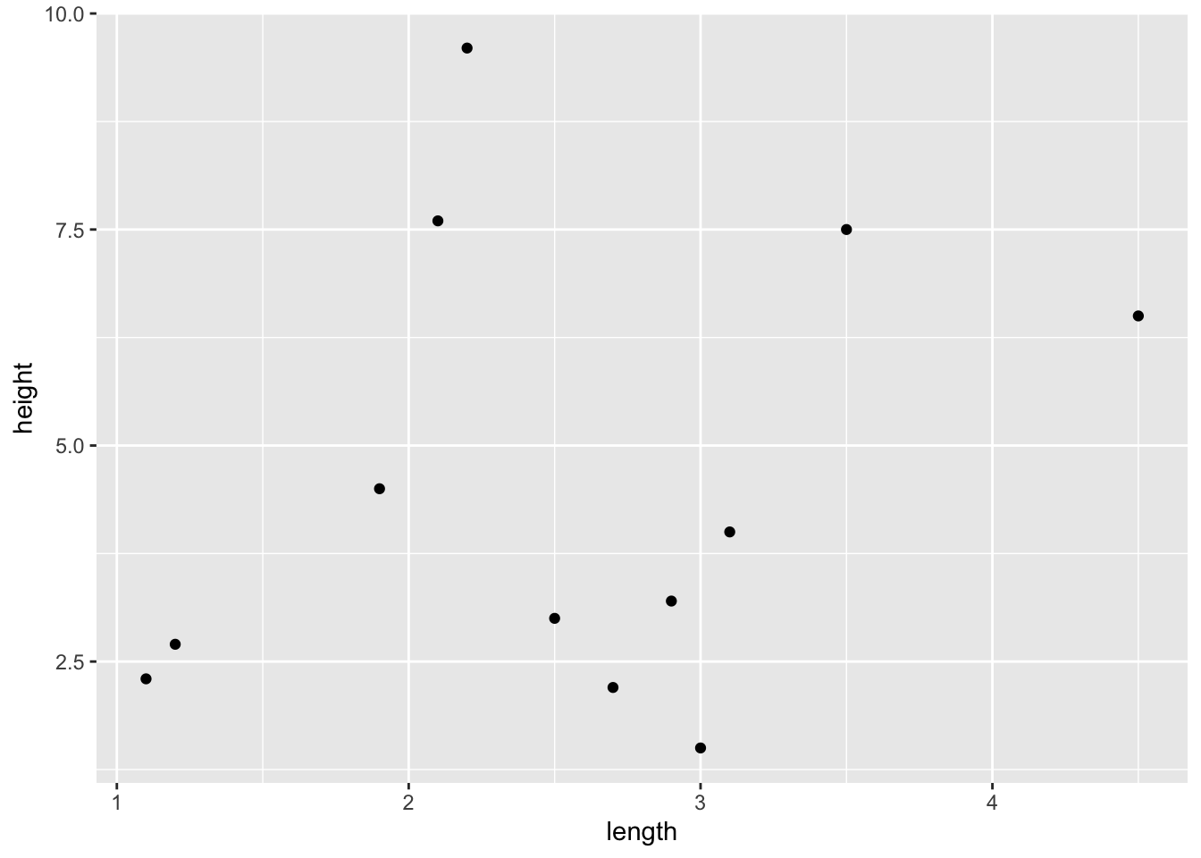
If you want to include a figure or image from outside RStudio, you can use the knitr::include_graphics() function (make sure you have installed the knitr package first). You simply need to specify the file directory for that figure. To include a figure caption, you can add this to the curly brackets at the start of the code chunk between ```{r and }.

Figure 17.3: R Studio Logo
17.4.5 Tables
Simple tables can be included using the following notation:
Column 1 Name | Column 2 Name
------------- | -------------
Cell 1        | Cell 2
Cell 3        | Cell 4
The output appears as follows:
| Column 1 Name | Column 2 Name |
|---|---|
| Cell 1 | Cell 2 |
| Cell 3 | Cell 4 |
Alternatively, if you want to include a larger table of data you can again use the knitr package, this time using the function knitr::kable(). This function allows you to directly specify the caption within kable(). For example, we can again use the ShrubData dataframe.
| site | experiment | length | width | height |
|---|---|---|---|---|
| 1 | 1 | 2.2 | 1.3 | 9.6 |
| 1 | 2 | 2.1 | 2.2 | 7.6 |
| 1 | 3 | 2.7 | 1.5 | 2.2 |
| 2 | 1 | 3.0 | 4.5 | 1.5 |
| 2 | 2 | 3.1 | 3.1 | 4.0 |
| 2 | 3 | 2.5 | 2.8 | 3.0 |
| 3 | 1 | 1.9 | 1.8 | 4.5 |
| 3 | 2 | 1.1 | 0.5 | 2.3 |
| 3 | 3 | 3.5 | 2.0 | 7.5 |
| 4 | 1 | 2.9 | 2.7 | 3.2 |
| 4 | 2 | 4.5 | 4.8 | 6.5 |
| 4 | 3 | 1.2 | NA | 2.7 |
17.5 Further Reading
Reference guide: https://www.rstudio.com/wp-content/uploads/2015/03/rmarkdown-reference.pdf?_ga=2.39431847.562324105.1650909679-1492771989.1650909679
R Markdown: The Definitive Guide by Xie et al.: https://bookdown.org/yihui/rmarkdown/